
Understanding when efficiency occurs, and its value at those times, is a central component of BTO’s efforts.
May 21, 2019
The Building Technologies Office (BTO) recently issued an article on the reasons why the timing of energy efficiency matters – we build electricity systems to meet peak demand, generation resources are economically dispatched, and the social cost of economic dispatch is not trivial. Today, we consider how much timing matters. Understanding when efficiency occurs, and its value at those times, is a central component of BTO’s efforts to make building loads more dispatchable and responsive to grid needs and provide benefits to building owners and occupants. All electricity customers can benefit from lower bills, and utilities and other grid operators benefit from reduced demand when it is most valuable, promoting a least-cost, reliable electricity system.
To understand the time-sensitive value of energy efficiency, we need to consider when an energy-efficiency measure saves energy (for example, the hours, days, and months) and the value of reducing energy consumption at that time.
Historically, quantification of efficiency benefits focused largely on the economic value of annual energy reductions. As the requirements for and complexity of a more flexible and resilient electricity system increase, all characteristics including peak demand impacts of energy efficiency must be considered in order to create a more reliable, affordable electricity system.
In the building sector, most end uses do not have a constant energy consumption profile, as shown in Figures 1 and 2. This is why energy-efficiency measures produce energy savings that vary over the course of the day and year.
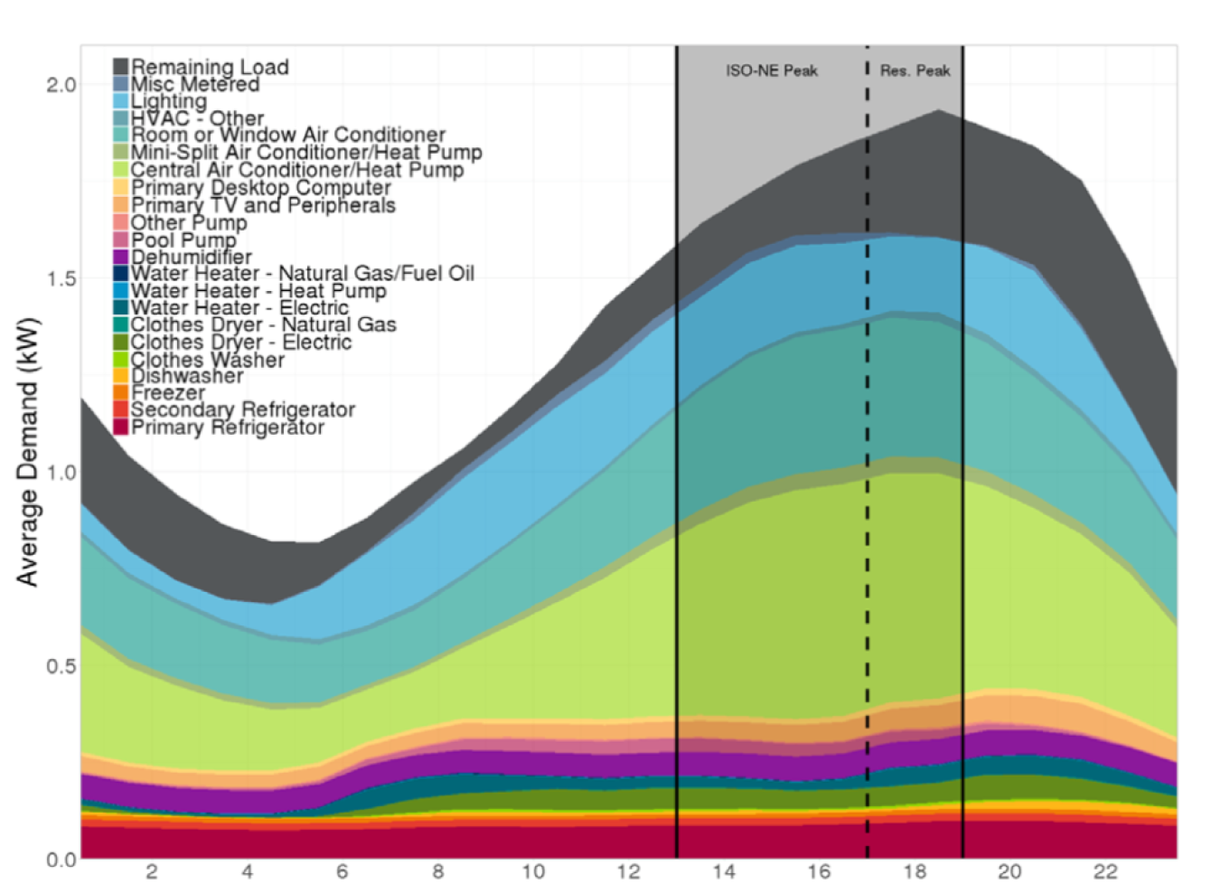
Figure 1. Massachusetts summer peak day end use load shapes (source: Navigant for the Electric and Gas Program Administrators of Massachusetts).

Figure 2. Massachusetts winter peak day end use load shapes (source: Navigant for the Electric and Gas Program Administrators of Massachusetts).
Similarly, the value of the hourly electricity savings varies because the avoided costs of generation, transmission, and distribution (T&D) are driven by a variety of influences. These factors include system congestion and the availability and cost of generation resources to meet loads at any given time. For example, ERCOT — the Independent System Operator that is responsible for the majority of Texas — has an energy-only market. This means that ERCOT uses only energy prices (not a capacity market like New England and PJM, for example) to ensure enough resources are built.
On typical days, prices are stable and relatively predictable. Figure 3 shows the average settlement prices for the ERCOT North Hub for March 2018. Most hours, the energy price is less than $25/megawatt-hour (MWh), and there are clear trends of when prices increase — when people wake up and are getting ready to leave the house, and again in the evening when offices are still humming but people are returning home. When compared to Figure 2, a winter peak day in New England, the overall shape is similar.
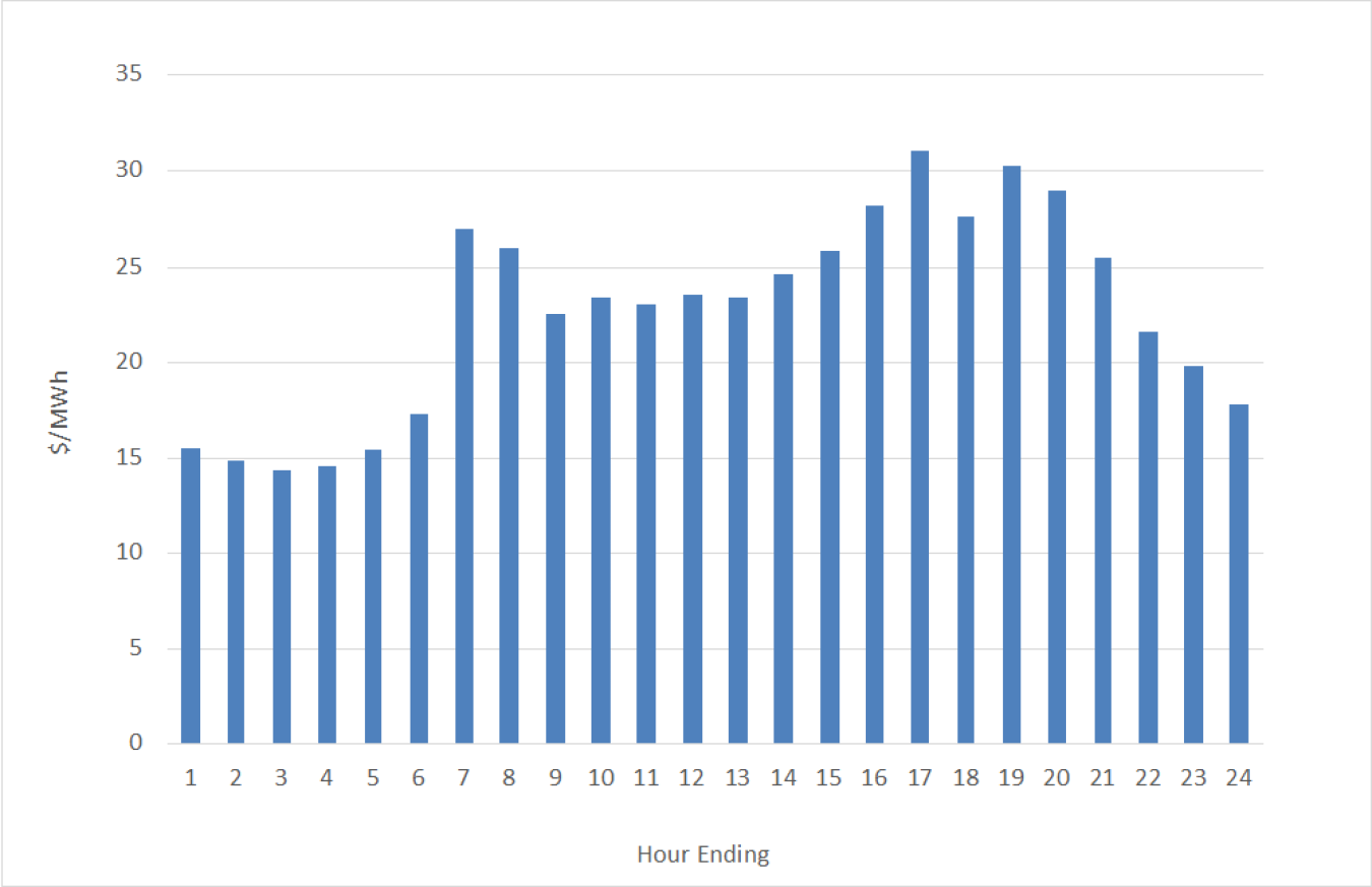
Figure 3. Average real-time market settlement prices at ERCOT North hub for March 2018 (source: ERCOT Historical Real Time Market Load Zone and Hub Prices).
However, a recent example of price volatility occurred in March 2019, when planned power plant maintenance and lower-than-expected wind generation resulted in an energy price spike, shown in Figure 4. Similar to the March 2018 pricing, in most hours the energy price was less than $25/MWh. However, from 7 to 8 a.m., the price spiked to over $382/MWh, more than a 15-fold leap. Examples like these clearly show that the value of reducing energy consumption at a given time has different values to the electricity system, both on a typical and an atypical day.
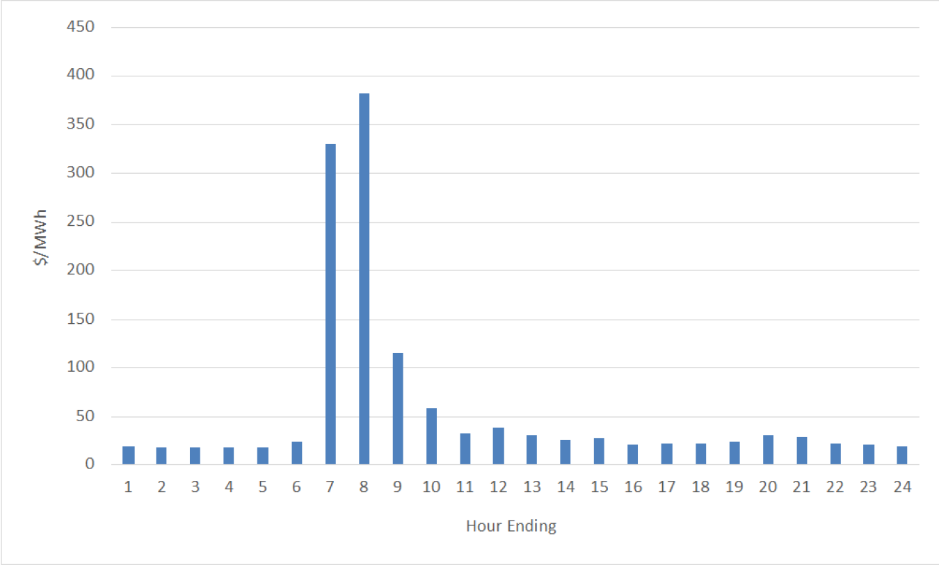
Figure 4. Real-time market settlement prices at ERCOT North hub on March 18, 2019 (source: ERCOT Historical Real Time Market Load Zone and Hub Prices).
To properly calculate the value of electricity savings to the utility system, it is necessary to account for time-related variations in energy savings and avoided cost. Information on energy savings may come from sources such as modeled end-use load profiles, advanced meter infrastructure (AMI) data, or submetering studies. Depending on the jurisdiction and market structure, avoided utility system costs might include:
- The cost of energy production at a given time
- Costs associated with the deferral of capital investment in new generation and T&D infrastructure
- Avoided costs of compliance with carbon dioxide and other emissions regulations
- Avoided renewable portfolio compliance costs
- Risk mitigation costs
- Demand reduction induced price effects
Lawrence Berkeley National Lab (Berkeley Lab), in partnership with the U.S. Department of Energy, is furthering research in this area. The main themes that have emerged from this research:
- The time-sensitive value of individual efficiency measures and how it varies across the locations studied
- Publicly available information on electric system costs avoided through energy efficiency that is not uniform across states and utilities
- Market structures and policies that play an important role in shaping the values used to calculate the time-sensitive value of efficiency
A recent report from Berkeley Lab released in 2018 assesses the time-sensitive value of five energy-efficiency measures (residential lighting, residential air-conditioning, residential water heating, commercial lighting and exit signs) in four states and one region: California, Georgia, Massachusetts, Michigan, and the Pacific Northwest region.
In Table 1, the time-varying value of residential air-conditioning savings in California and Massachusetts (which is highly coincident with both system’s summer peak demand) is nearly twice that of residential lighting, which peaks much later in the day in California and in Massachusetts. Comparatively, in the Pacific Northwest, which has a winter peak, the value of residential lighting is nearly twice that of residential air conditioning. In Georgia, where publicly available data did not include avoided T&D system values, the calculated time-varying value of efficiency appears to be much lower.
Table 1. Time-varying value of energy efficiency for five measures in four regions (2016$/MWh)
| Pacific NW | California | Massachusetts | Georgia | |
|---|---|---|---|---|
| EXIT SIGN | 89 | 90 | 169 | 41 |
| WATER HEATING | 103 | 92 | 166 | 43 |
| RESIDENTIAL AIR CONDITIONING | 67 | 208 | 371 | 67 |
| RESIDENTIAL LIGHTING | 116 | 107 | 179 | 42 |
| COMMERCIAL LIGHTING | 100 | 90 | 183 | 45 |
In doing the research for a 2018 white paper, Time-Varying Value of Energy Efficiency in Michigan, it became clear that the energy-efficiency measure assumptions had an impact on the value of each efficiency measure we analyzed. Figure 5 shows the ratio of the total time-varying value of electric efficiency measures (avoided cost of energy plus the avoided cost of capacity) to the energy-related value of savings for the energy efficiency measures under three sets of assumptions. For some measures, such as commercial lighting, the assumptions changed the value of savings by about 40%.

Figure 5. Ratio of total time-varying value of energy savings to energy-related savings value, by measure with three savings assumptions.
Understanding when efficiency occurs, and its value at those times, is a central component of BTO’s efforts to make building loads more dispatchable and responsive to grid needs and provide benefits to building owners and occupants. All electricity customers can benefit from lower bills, and utilities and other grid operators benefit from reduced demand when it is most valuable, promoting a least-cost, reliable electricity system.
Stay tuned for a future report from Berkeley Lab highlighting examples of utilities, regulators, and state energy offices taking the time-sensitive value of efficiency into account.
Read more in the Grid-interactive Efficient Buildings article series.